Using xG data from FBref
Using the acciotables API, and some minor data transformation in R, it’s possible to get Statsbomb/FBref expected goals data for every EPL match since 2017-18.
This standalone guide will produce a dataset and visualisation to use as a starting point for more detailed analysis and graphics. You don’t need your own data, just an installation of R and RStudio.
Getting data with the acciotables API
FBref stores a summary of all 380 matches in a single html table. We just need the page_url and selector_id, and acciotables will produce the data in a nice html format.
Looking in the page source gives the selector_id: %23sched_ks_3232_1
page_url <- "https://fbref.com/en/comps/9/3232/schedule/"
selector_id <- "%23sched_ks_3232_1"
url <- paste0("http://acciotables.herokuapp.com/?page_url=",page_url,"&content_selector_id=",selector_id)

cat(paste0("API url: ",url))
## API url: http://acciotables.herokuapp.com/?page_url=https://fbref.com/en/comps/9/3232/schedule/&content_selector_id=%23sched_ks_3232_1
Check the API is working in your browser.
Importing into R
There’s a guide in the acciotables readme.
matches_import <- url %>%
  read_html() %>%
  html_table() %>%
  extract2(1) # unnest the data_frame from the list

head(matches_import)
##   Wk Day       Date          Time           Home  xG Score  xG            Away
## 1  1 Fri 2019-08-09 20:00 (19:00)      Liverpool 1.7   4–1 1.0    Norwich City
## 2  1 Sat 2019-08-10 12:30 (11:30)       West Ham 0.8   0–5 3.1 Manchester City
## 3  1 Sat 2019-08-10 15:00 (14:00)        Burnley 0.7   3–0 0.8     Southampton
## 4  1 Sat 2019-08-10 15:00 (14:00)        Watford 0.9   0–3 0.7        Brighton
## 5  1 Sat 2019-08-10 15:00 (14:00)    Bournemouth 1.0   1–1 1.0   Sheffield Utd
## 6  1 Sat 2019-08-10 15:00 (14:00) Crystal Palace 0.7   0–0 1.0         Everton
##   Attendance                 Venue        Referee Match Report Notes
## 1     53,333               Anfield Michael Oliver Match Report
## 2     59,870        London Stadium      Mike Dean Match Report
## 3     19,784             Turf Moor   Graham Scott Match Report
## 4     20,245 Vicarage Road Stadium   Craig Pawson Match Report
## 5     10,714      Vitality Stadium   Kevin Friend Match Report
## 6     25,151         Selhurst Park  Jonathan Moss Match Report
Tidy the data
There’s a few things to sort out to make the raw data more usable.
- There are two columns called
xG. That is definitely going to make something go wrong.
names(matches_import) <-
  names(matches_import) %>%
  make.unique(sep="_")

matches_tidy1 <-
  matches_import %>%
  rename("HomexG"="xG","AwayxG"="xG_1")

gt(head(matches_tidy1))
| Wk | Day | Date | Time | Home | HomexG | Score | AwayxG | Away | Attendance | Venue | Referee | Match Report | Notes |
|---|---|---|---|---|---|---|---|---|---|---|---|---|---|
| 1 | Fri | 2019-08-09 | 20:00 (19:00) | Liverpool | 1.7 | 4–1 | 1.0 | Norwich City | 53,333 | Anfield | Michael Oliver | Match Report | |
| 1 | Sat | 2019-08-10 | 12:30 (11:30) | West Ham | 0.8 | 0–5 | 3.1 | Manchester City | 59,870 | London Stadium | Mike Dean | Match Report | |
| 1 | Sat | 2019-08-10 | 15:00 (14:00) | Burnley | 0.7 | 3–0 | 0.8 | Southampton | 19,784 | Turf Moor | Graham Scott | Match Report | |
| 1 | Sat | 2019-08-10 | 15:00 (14:00) | Watford | 0.9 | 0–3 | 0.7 | Brighton | 20,245 | Vicarage Road Stadium | Craig Pawson | Match Report | |
| 1 | Sat | 2019-08-10 | 15:00 (14:00) | Bournemouth | 1.0 | 1–1 | 1.0 | Sheffield Utd | 10,714 | Vitality Stadium | Kevin Friend | Match Report | |
| 1 | Sat | 2019-08-10 | 15:00 (14:00) | Crystal Palace | 0.7 | 0–0 | 1.0 | Everton | 25,151 | Selhurst Park | Jonathan Moss | Match Report |
- The dataset has some non-data lines. There should be 380 lines of data, one for each match in the season.
matches_tidy2 <-
  matches_tidy1 %>%
  filter(Wk!="Wk",Wk!="")

cat(paste0("rows: ",dim(matches_tidy2)[1],"\n","columns: ",dim(matches_tidy2)[2]))
## rows: 380
## columns: 14
- Don’t care about the attendance, referee etc.
matches_tidy3 <-
  matches_tidy2 %>%
  select(-c("Attendance":"Notes"))

gt(head(matches_tidy3))
| Wk | Day | Date | Time | Home | HomexG | Score | AwayxG | Away |
|---|---|---|---|---|---|---|---|---|
| 1 | Fri | 2019-08-09 | 20:00 (19:00) | Liverpool | 1.7 | 4–1 | 1.0 | Norwich City |
| 1 | Sat | 2019-08-10 | 12:30 (11:30) | West Ham | 0.8 | 0–5 | 3.1 | Manchester City |
| 1 | Sat | 2019-08-10 | 15:00 (14:00) | Burnley | 0.7 | 3–0 | 0.8 | Southampton |
| 1 | Sat | 2019-08-10 | 15:00 (14:00) | Watford | 0.9 | 0–3 | 0.7 | Brighton |
| 1 | Sat | 2019-08-10 | 15:00 (14:00) | Bournemouth | 1.0 | 1–1 | 1.0 | Sheffield Utd |
| 1 | Sat | 2019-08-10 | 15:00 (14:00) | Crystal Palace | 0.7 | 0–0 | 1.0 | Everton |
- The
Scorecolumn looks something like 4-1. We want two columns: home goals and away goals.
matches_tidy4 <-
  matches_tidy3 %>%
  separate("Score",c("HomeGls","AwayGls"),sep="[:punct:]",fill="right")

gt(head(matches_tidy4))
| Wk | Day | Date | Time | Home | HomexG | HomeGls | AwayGls | AwayxG | Away |
|---|---|---|---|---|---|---|---|---|---|
| 1 | Fri | 2019-08-09 | 20:00 (19:00) | Liverpool | 1.7 | 4 | 1 | 1.0 | Norwich City |
| 1 | Sat | 2019-08-10 | 12:30 (11:30) | West Ham | 0.8 | 0 | 5 | 3.1 | Manchester City |
| 1 | Sat | 2019-08-10 | 15:00 (14:00) | Burnley | 0.7 | 3 | 0 | 0.8 | Southampton |
| 1 | Sat | 2019-08-10 | 15:00 (14:00) | Watford | 0.9 | 0 | 3 | 0.7 | Brighton |
| 1 | Sat | 2019-08-10 | 15:00 (14:00) | Bournemouth | 1.0 | 1 | 1 | 1.0 | Sheffield Utd |
| 1 | Sat | 2019-08-10 | 15:00 (14:00) | Crystal Palace | 0.7 | 0 | 0 | 1.0 | Everton |
- All the data has the character datatype.
type_convertwill handily auto-detect which ones should be numeric, date etc.
matches_tidy5 <-
  matches_tidy4 %>%
  type_convert()
This is much easier to work with, but there’s one more change that will help a lot later.
Transform into long data
Tidy data has one observation per row. Each line in this table has two independent(ish) observations: home score and away score. By transforming to long (as opposed to wide) format, working with the data becomes much easier.
What’s happening here:
pivot_longerto separate home and away into two rows.- The original
matchesdata frame joined back to the new data - a bit of a trick to get a sort of metadata, for filtering or labelling. Don’t worry too much about this if it doesn’t make sense. - Then
if_elseto sort out the rest of the home/away data. relocatethe columns used in the final plot to the left to make it easier to see.
This is a useful transformation, so it’s all in a function called make_long_matches.
make_long_matches <- function(matches){

  long_matches <-
    matches %>%
    pivot_longer(cols=c(Home,Away),
                 names_to="HA",
                 values_to="Squad") %>%
    left_join(matches) %>% # join the old data frame to the new one
    mutate(
      Opposition=ifelse(HA=="Home",Away,Home),
      GlsF=ifelse(HA=="Home",HomeGls,AwayGls),
      GlsA=ifelse(HA=="Home",AwayGls,HomeGls),
      xGF=ifelse(HA=="Home",HomexG,AwayxG),
      xGA=ifelse(HA=="Home",AwayxG,HomexG)
    ) %>%
    relocate("Squad","Opposition":"xGA","HA")

  return(long_matches)
}

matches_long <- make_long_matches(matches_tidy5)

gt(head(matches_long))
| Squad | Opposition | GlsF | GlsA | xGF | xGA | HA | Wk | Day | Date | Time | HomexG | HomeGls | AwayGls | AwayxG | Home | Away |
|---|---|---|---|---|---|---|---|---|---|---|---|---|---|---|---|---|
| Liverpool | Norwich City | 4 | 1 | 1.7 | 1.0 | Home | 1 | Fri | 2019-08-09 | 20:00 (19:00) | 1.7 | 4 | 1 | 1.0 | Liverpool | Norwich City |
| Norwich City | Liverpool | 1 | 4 | 1.0 | 1.7 | Away | 1 | Fri | 2019-08-09 | 20:00 (19:00) | 1.7 | 4 | 1 | 1.0 | Liverpool | Norwich City |
| West Ham | Manchester City | 0 | 5 | 0.8 | 3.1 | Home | 1 | Sat | 2019-08-10 | 12:30 (11:30) | 0.8 | 0 | 5 | 3.1 | West Ham | Manchester City |
| Manchester City | West Ham | 5 | 0 | 3.1 | 0.8 | Away | 1 | Sat | 2019-08-10 | 12:30 (11:30) | 0.8 | 0 | 5 | 3.1 | West Ham | Manchester City |
| Burnley | Southampton | 3 | 0 | 0.7 | 0.8 | Home | 1 | Sat | 2019-08-10 | 15:00 (14:00) | 0.7 | 3 | 0 | 0.8 | Burnley | Southampton |
| Southampton | Burnley | 0 | 3 | 0.8 | 0.7 | Away | 1 | Sat | 2019-08-10 | 15:00 (14:00) | 0.7 | 3 | 0 | 0.8 | Burnley | Southampton |
cat(paste0("rows: ",dim(matches_long)[1],"\n","columns: ",dim(matches_long)[2]))
## rows: 760
## columns: 17
Now there are 760 rows, one for each team in each match.
Filter
Next the data can be filtered get a subset for analysis. In this case it’s the data for all matches played so far by a single team.
team_name <- "Liverpool"

matches_team <-
  matches_long %>%
  filter(Squad==team_name) %>% # filter team
  filter(!is.na(HomeGls)) # only matches which have been played
Some work to use later - create an new column to use as an X axis label, and use fct_reorder to get the X axis in date order.
matches_team <-
  matches_team %>%
  mutate(Match=paste0(Opposition," ",HA," ",GlsF,"-",GlsA)) %>% # make X axis labels
  mutate(Match=fct_reorder(Match, Date)) # order by date
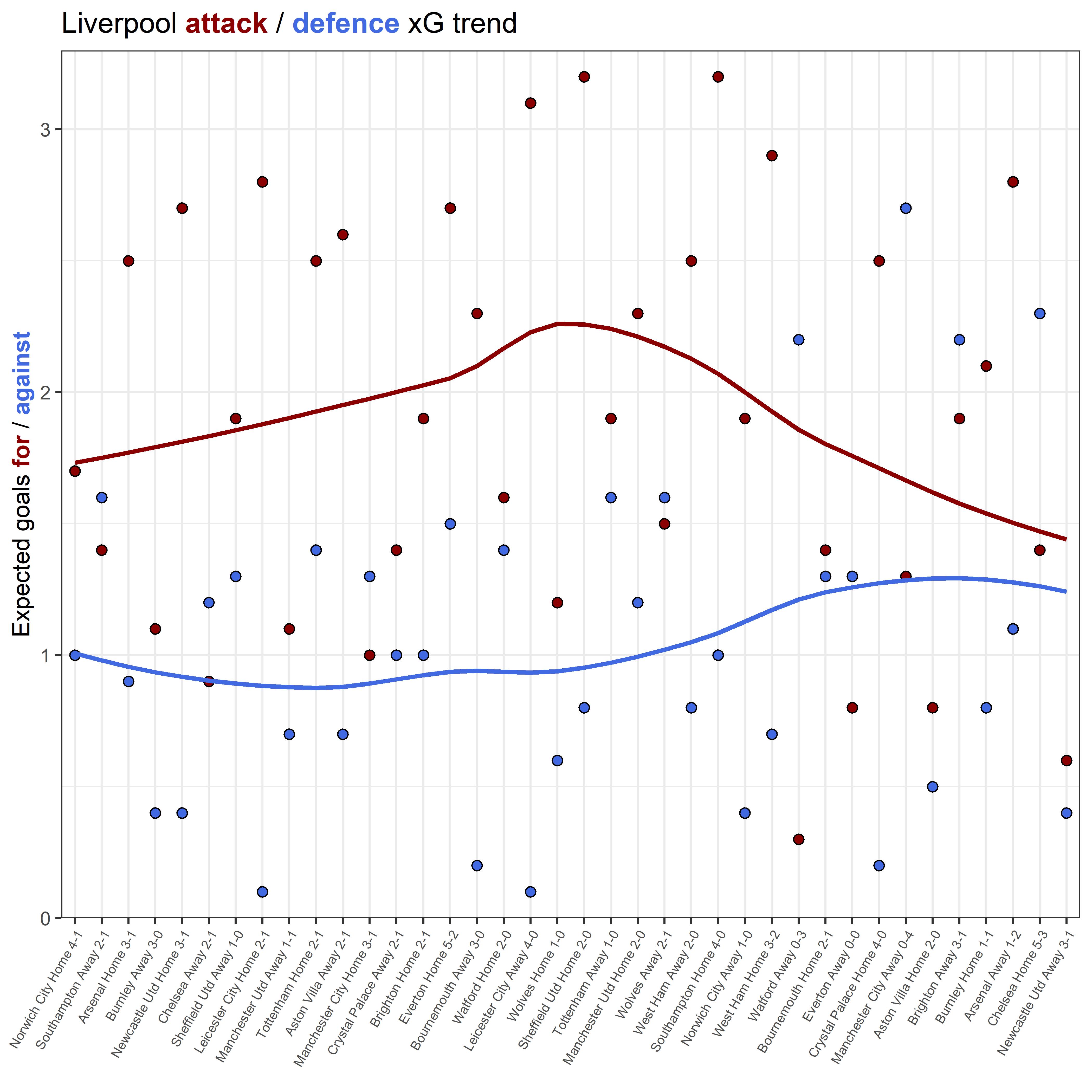
Plot
Lots of ways to do this, here’s a ggplot with some lines, some points, a theme, and some slightly better labels made with ggtext.
matches_team %>%
  ggplot(aes(x=Match,group=1)) +
  geom_point(aes(y=xGF),size=2,colour="black",fill="darkred",shape=21) +
  geom_smooth(aes(y=xGF),colour="darkred",se=FALSE) +
  geom_point(aes(y=xGA),size=2,colour="black",fill="royalblue",shape=21) +
  geom_smooth(aes(y=xGA),colour="royalblue",se=FALSE) +
  theme_bw() +
  theme(
    plot.title=element_markdown(),
    axis.title.y=element_markdown(),
    axis.text.x=element_text(size=6,angle=60,hjust=1)
  ) +
  labs(
    title=paste0(team_name," <b style='color:darkred'>attack</b> / <b style='color:royalblue'>defence</b> xG trend"),
    x=element_blank(),
    y=("Expected goals <b style='color:darkred'>for</b> / <b style='color:royalblue'>against</b>")
  ) +
  scale_x_discrete(expand=expansion(add=c(0.5))) +
  scale_y_continuous(limits=c(0,NA),expand=expansion(add=c(0,0.1)))
Further reading / references / acknowledgements
- Complete script - this is compressed a bit more and uses moving averages on the same data.
- RMarkdown script used to create this post.
- acciotables by Pranav N
- ggtext for Markdown in ggplots
- Statsbomb for providing the data hosted by FBref
- R Graph Gallery and Cédric Scherer for more viz ideas
- Need help? Probably best to tweet at me
One more thing
It’s friendly to give credit to the data providers at Statsbomb and FBref. Statsbomb’s media guide is here, and if you want to add their logos to your images, you can use Cowplot for that.