Distinct passing profiles in Statsbomb 360 data

The concepts in this post are extensively borrowed from Andy Rowlinson’s work.

Isolation Forest algorithm for Statsbomb 360 data

Statsbomb have released Women’s Euro 2022 event data alongside their Men’s Euro 2020 data, presenting a good opportunity for some Machine Learning analysis on a rich event dataset.

Andy Rowlinson demonstrated an Isolation Forest algorithm using Euro 2022 passing data, as a method to answer the question: “which players have the most unusual passing profiles”. This blog reimplements that approach using R.

R code for this blog

What does an Isolation Forest do?

An Isolation Forest algorithm identifies anomalies in a dataset. The image below shows anomaly scores for a two-dimensional dataset, with greater anomalies in darker red.

Isolation Forest Wiki

An Isolation Forest generalises this to identify outliers in data with many dimensions.

Packages

library(tidyverse)
library(StatsBombR)
library(ggsoccer)
library(isotree)

StatsBombR package installation guide

The isotree R package is used to create the Isolation Forest model, because it is the most useable model I can find that isn’t specifically designed for time series data.

Data import

FreeCompetitions <- FreeCompetitions()

Euro2022 <- FreeCompetitions %>%
  filter(competition_id==53)

Euro2022Matches <- FreeMatches(Euro2022)
Euro2022Events <- free_allevents(MatchesDF=Euro2022Matches, Parallel=T) %>% allclean()

Import following the StatsBomb Working with R guide.

Pre-processing

passes <-
  Euro2022Events %>%
  # filter pass events
  filter(type.name %in% c("Pass")) %>% 
  # remove set piece pass types
  filter(!(pass.type.name %in% c("Kick Off","Goal Kick","Corner","Throw-in","Free Kick"))) %>%
  # keep player name and pass location
  select(
    player.name,
    location.x,location.y,
    pass.end_location.x,pass.end_location.y
  ) %>%
  # bin into pitch zones
  mutate(
    # treat the defensive half as one zone
    # split the attacking half into 20 x 20 zones
    across(where(is.numeric) & contains("x"),cut,breaks=c(0,60,80,100,120),.names="{.col}.bin"),
    across(where(is.numeric) & contains("y"),cut,breaks=seq(0,80,20),.names="{.col}.bin"),
	across(contains(".bin"),as.character)
  ) %>%
  mutate(
    # single y axis zone for the defensive half
    location.y.bin=ifelse(location.x.bin=="(0,60]","(0,80]",location.y.bin),
    pass.end_location.y.bin=ifelse(pass.end_location.x.bin=="(0,60]","(0,80]",pass.end_location.y.bin),
  )

  player.name           location.y location.y.bin
  <chr>                      <dbl> <chr>         
Sarah Puntigam              45.2 (0,80]        
Viktoria Schnaderbeck       37.6 (0,80]        
Carina Wenninger            66.7 (0,80]        
Rachel Daly                 13.6 (0,80]        
Sarah Zadrazil              63.4 (60,80]       
Nicole Billa                57.1 (40,60]       
Barbara Dunst               51.5 (40,60]       
Laura Feiersinger           37.8 (20,40]

(location.y and location.y.bin columns only)

This creates a data frame of passes containing: player name, pass start location and pass end location.

In StatsBomb data, the pitch has dimensions of 120x80. The Isolation Forest requires categorised data, so the start and end locations are binned into:

A 20x20 grid in the attacking half (4 squares wide and 3 squares long)
A single bin in the defensive half

# count the total number of passes by each player
passes_total <-
  passes %>%
  group_by(player.name) %>%
  summarise(passes=n(),.groups="drop") %>%
  arrange(desc(passes))

   player.name                 passes
   <chr>                        <int>
Leah Williamson                522
María Pilar León Cebrián       393
Keira Walsh                    359
Irene Paredes Hernandez        351
Millie Bright                  347

Passing totals are useful to have for later.

Transition matrix

transition_matrix <-
  passes %>%
  group_by(player.name,across(contains(".bin"))) %>%
  summarise(passes=n(),.groups="drop") %>%
  pivot_wider(
    names_from = c(location.x.bin,location.y.bin,pass.end_location.x.bin,pass.end_location.y.bin),
	names_sort = TRUE,
    values_from = passes,
    values_fill = 0
  )

Rows: 308
Columns: 146
$ player.name                       <chr> "Abbie Magee", "Ada Stolsmo Hegerberg", "Adelina Engman", "Agla Marí…
$ `(0,60]_(0,80]_(0,60]_(0,80]`     <int> 15, 12, 7, 7, 6, 70, 70, 7, 48, 5, 17, 1, 20, 93, 0, 11, 1, 13, 19, …
$ `(0,60]_(0,80]_(100,120]_(0,20]`  <int> 0, 0, 0, 0, 0, 0, 0, 0, 2, 0, 1, 0, 0, 0, 0, 0, 0, 0, 0, 0, 0, 0, 2,…
$ `(0,60]_(0,80]_(100,120]_(20,40]` <int> 0, 0, 0, 0, 0, 0, 0, 0, 2, 0, 0, 0, 0, 0, 0, 0, 0, 0, 0, 0, 0, 0, 1,…
$ `(0,60]_(0,80]_(100,120]_(40,60]` <int> 0, 0, 0, 0, 0, 0, 0, 0, 0, 0, 0, 0, 0, 2, 0, 0, 0, 0, 0, 0, 0, 0, 1,…
$ `(0,60]_(0,80]_(100,120]_(60,80]` <int> 1, 0, 0, 0, 0, 2, 0, 1, 0, 0, 0, 0, 0, 0, 0, 0, 0, 0, 0, 0, 0, 0, 0,…
$ `(0,60]_(0,80]_(60,80]_(0,20]`    <int> 0, 1, 0, 1, 0, 1, 4, 0, 5, 0, 3, 0, 0, 1, 0, 2, 0, 0, 0, 4, 4, 0, 7,…

(matrix transposed with glimpse - player names are the rows, columns are coordinates in x_y_xend_yend format. Matrix view.

This section creates a data frame transition_matrix of players (308 rows) and start/end pass zones (146 columns), counting the proportion of passes starting and ending in each zone.

Many passes begin and end in the defensive half, represented by the (0,60]_(0,80]_(0,60]_(0,80] category.

transition_matrix_normal <-
  transition_matrix %>%
  # join total passes column
  inner_join(passes_total) %>%
  # divide by total player passes to normalise rows
  mutate(across(!c(player.name,passes),~.x/passes))

Rows: 308
Columns: 146
$ player.name                       <chr> "Abbie Magee", "Ada Stolsmo Hegerberg", "Adelina Engman", "Agla Marí…
$ `(0,60]_(0,80]_(0,60]_(0,80]`     <dbl> 0.484, 0.207, 0.318, 0.318, 0.333, 0.737, 0.235, 0.156, 0.338, 0.556…
$ `(0,60]_(0,80]_(100,120]_(0,20]`  <dbl> 0.000, 0.000, 0.000, 0.000, 0.000, 0.000, 0.000, 0.000, 0.014, 0.000…
$ `(0,60]_(0,80]_(100,120]_(20,40]` <dbl> 0.000, 0.000, 0.000, 0.000, 0.000, 0.000, 0.000, 0.000, 0.014, 0.000…
$ `(0,60]_(0,80]_(100,120]_(40,60]` <dbl> 0.000, 0.000, 0.000, 0.000, 0.000, 0.000, 0.000, 0.000, 0.000, 0.000…
$ `(0,60]_(0,80]_(100,120]_(60,80]` <dbl> 0.032, 0.000, 0.000, 0.000, 0.000, 0.021, 0.000, 0.022, 0.000, 0.000…
$ `(0,60]_(0,80]_(60,80]_(0,20]`    <dbl> 0.000, 0.017, 0.000, 0.045, 0.000, 0.011, 0.013, 0.000, 0.035, 0.000…

(matrix transposed with glimpse - rows are player names, columns are coordinates in x_y_xend_yend format) Matrix view.

The data is normalised to the interval [0,1] by dividing by the total number of passes per player. This ensures that total pass volume does not effect whether a pass profile is distinct.

Isolation Forest training

# create isolation forest using isotree function
forest <-
  transition_matrix_normal %>%
  select(-player.name,-passes) %>%
  isolation.forest(
    data=.,
    ndim=1,
    ntree=500,
    missing_action="fail",
    scoring_metric="density"
  )

The Isolation Forest is trained on the transition matrix. 500 trees is sufficient to give repeatable results.

I have replicated the approach in the isotree Isolation Forest guide to train this model, mostly the example with real data which trains the Isolation Forest on a large matrix.

Prediction

# calculate the isolation prediction of each player
prediction <-
  # join the prediction to the transition matrix containing player names
  bind_cols(
    # predict using isotree function
    predict(forest, transition_matrix_normal) %>%
      tibble("anomaly_score"=.),
    # join to transition matrix
    transition_matrix_normal
  ) %>%
  # keep the player name and prediction
  select(player.name,anomaly_score) %>%
  # join the player passes total
  inner_join(passes_total) %>%
  # only keep players with at least 20 passes
  filter(passes >= 20) %>%
  # order by prediction
  arrange(desc(anomaly_score))

   player.name                            anomaly_score passes
   <chr>                                          <dbl>  <int>
Francisca Ramos Ribeiro Nazareth Sousa         -4.78     31
Aitana Bonmati Conca                           -5.06    298
Jill Roord                                     -5.09    134
Ella Toone                                     -5.23    130
Barbara Bonansea                               -5.25     56
Andreia Alexandra Norton                       -5.37     98
Bethany Mead                                   -5.40    145
Charlotte Bilbault                             -5.40    187
Nicole Billa                                   -5.45     80
María Francesca Caldentey Oliver               -5.56    273
Cristiana Girelli                              -5.56     58
Lea Schüller                                   -5.67     29

The anomaly score of each player pass profile is calculated. The isotree::predict function creates an array of predictions which corresponds to the players in the isolatioin matrix, joined back to the matrix with bind_cols.

Players with higher (closer to zero) anomaly_score are the most isolated profiles identified by the algorithm.

Results

# inner join to only keep player data from the top 12 predictions
inner_join(
  passes,
  prediction %>%
    slice_max(anomaly_score,n=12)
) %>%
  # wrap longer names
  mutate(player.name=str_wrap(player.name,width=25)) %>%
  # order by ranking
  mutate(player.name=fct_reorder(player.name,desc(anomaly_score))) %>%
  ggplot() +
  annotate_pitch(dimensions=pitch_statsbomb) +
  geom_segment(aes(x=location.x,xend=pass.end_location.x,y=location.y,yend=pass.end_location.y),size=0.3,arrow=arrow(length=unit(0.1, "cm"))) +
  theme_pitch() +
  theme(
    strip.text=element_text(size=6),
    strip.background=element_blank(),
    plot.caption=element_text(face="italic",size=6)
  ) +
  facet_wrap(vars(player.name),ncol=4) +
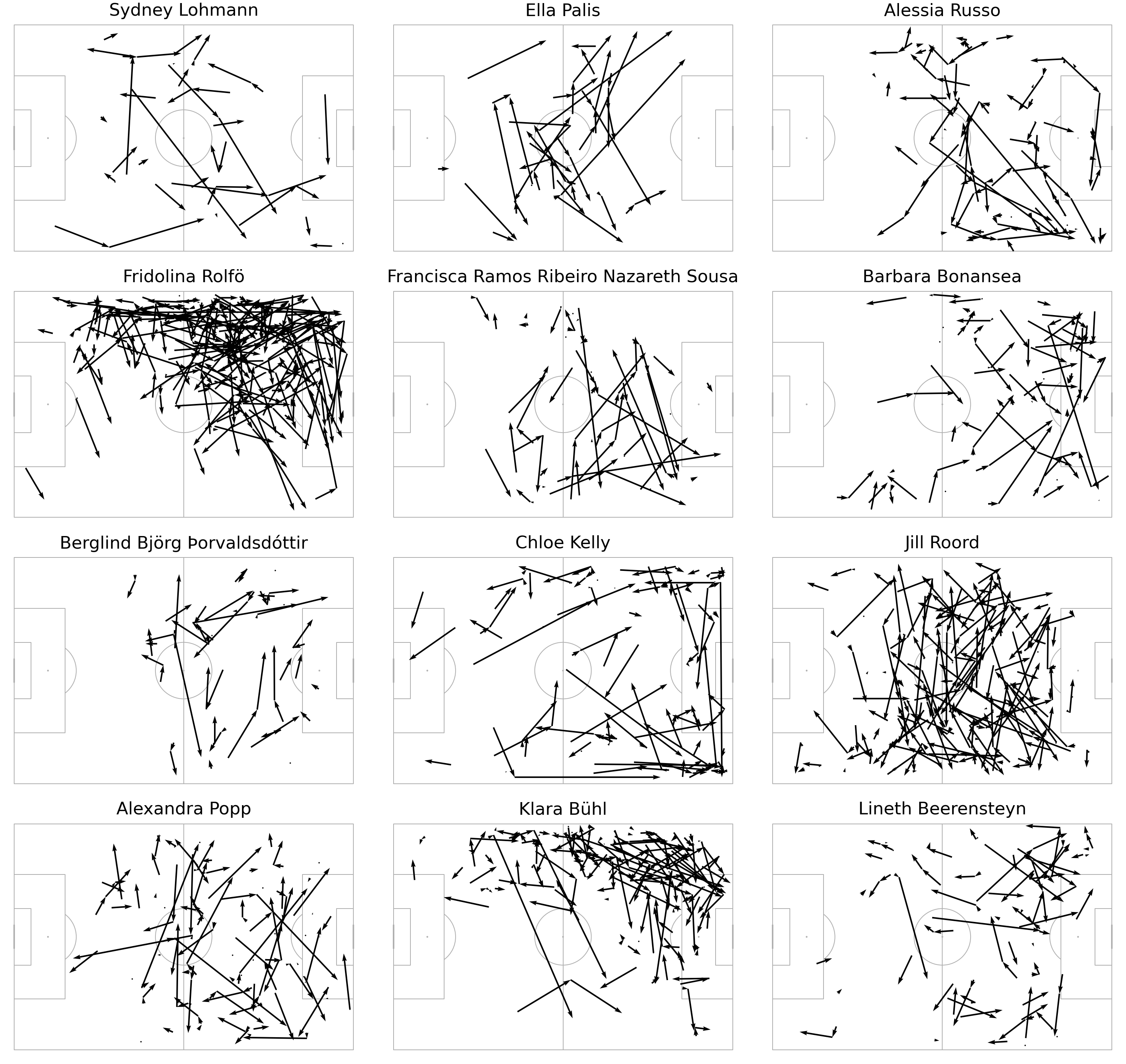
  labs(
    title="Most unique Euro 2022 passing profiles",
    caption="Statsbomb 360 data"
  )

Congratulations to Francisca Nazareth of Portugal, whose 31 passes were more distinct than some more well-known creative passers such as Aitana Bonmatí (pictured above).

Three players identified in this implementation also appeared in Andy’s implementation:

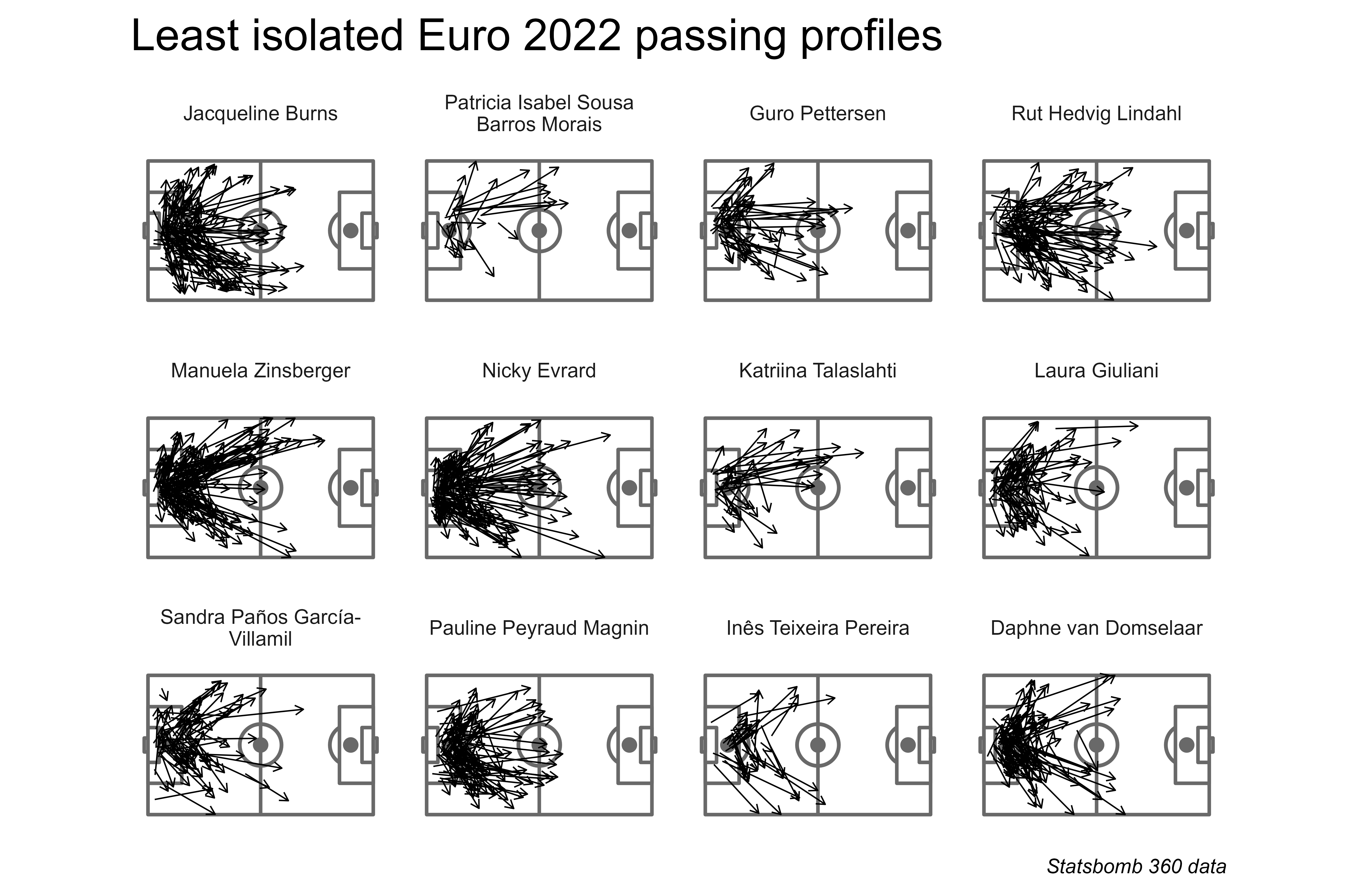
Naturally, the least isolated set of players were mostly goalkeepers. Grouping the defensive half as a single zone helps to differentiate attacking passers over defensive ones.

What about testing the algorithm with Men’s Euro 2020 data?

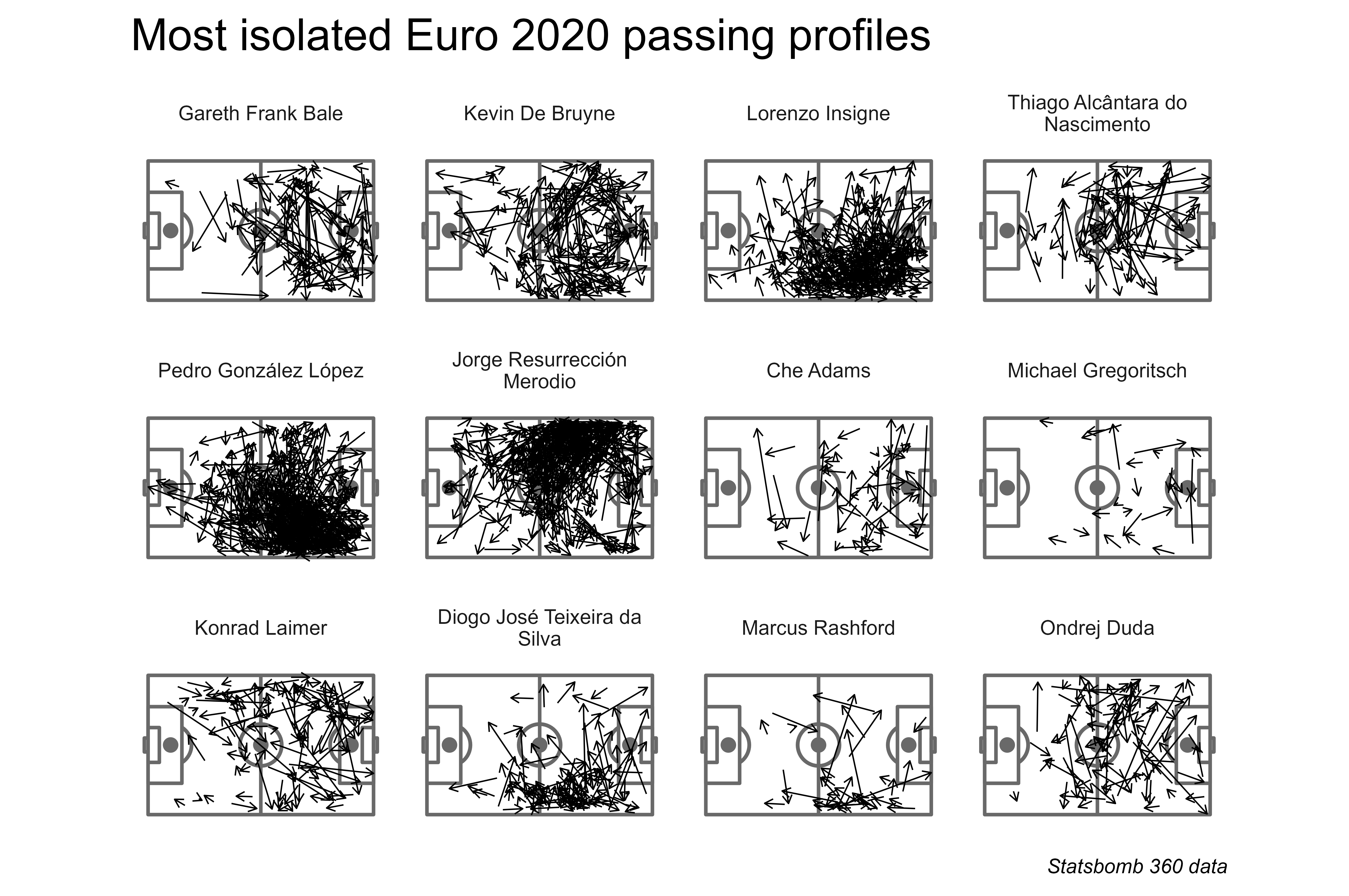
It’s notable that some players who carried a lot of their country’s passing have the most distinct passing profiles with this algorithm.

Limitations

Players who didn’t progress through the knockout stages have limited passing data.
Distinct passing profile may not indicate actual passing ability.
Zones are discrete features and the model doesn’t know which zones are adjacent.
Passing location is affected by teams playing higher or lower lines.
Players who can play in multiple positions (such as on both wings) are over-identified, even if their actual passing characteristics are typical for wide players.
Midfield passers from just inside the attacking half may be over-identified.
Progressive passers from some deep positions may be under-identified.
Passers into very dangerous penalty area positions may be under-identified.

Thanks to

Andy Rowlinson for sharing his original work and allowing me to borrow his ideas to reproduce in R (mistakes are mine).
StatsBomb for providing Euro 2022 and Euro 2020 event data.
David Cortes, creator of isotree.
Ben Torvaney, creator of ggsoccer.

Questions, comments and complaints to:

saintsbynumbers@gmail.com
@saintsbynumbers on Twitter
szfh on Github

Written on August 14, 2022